mundial-2026-ml
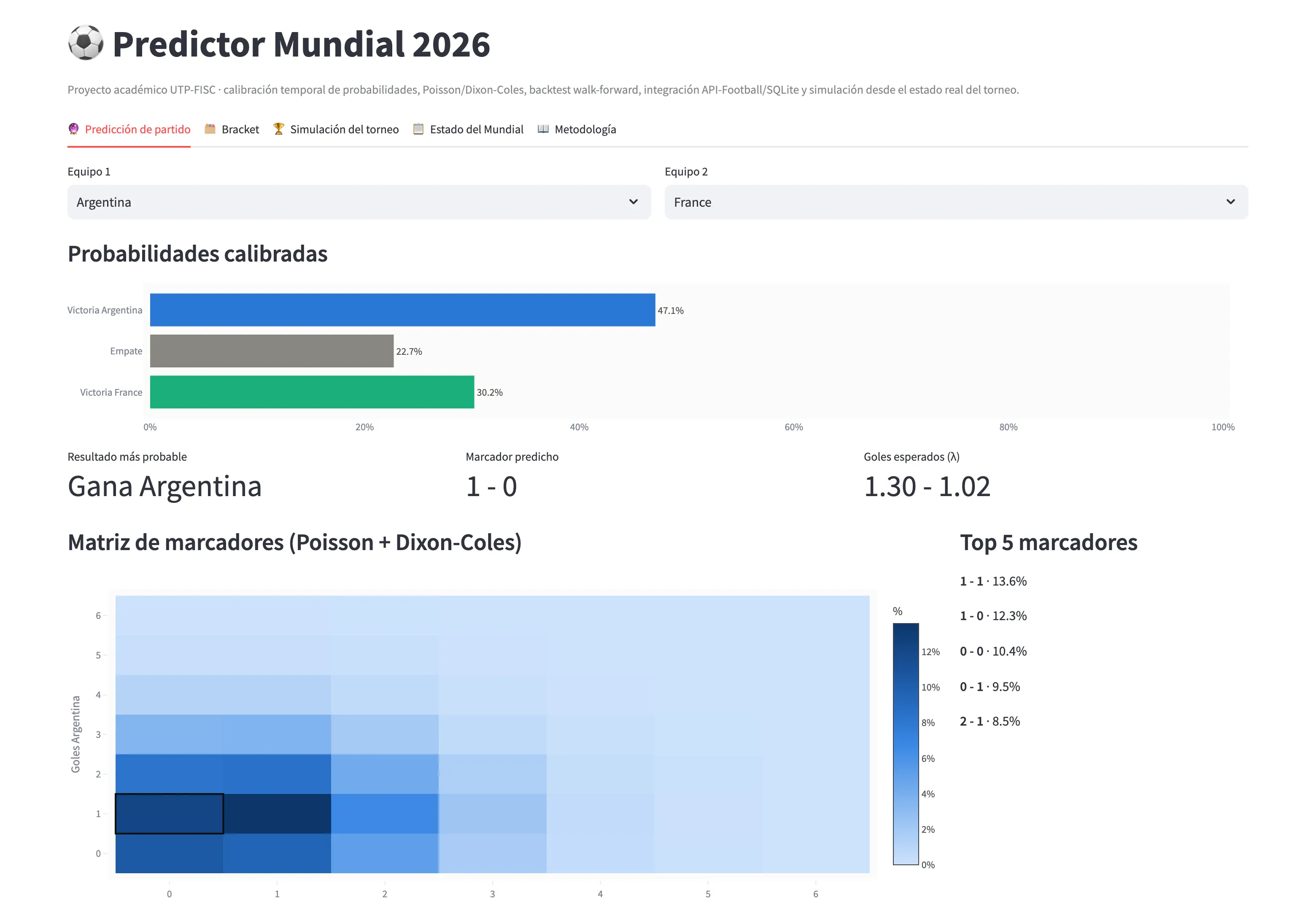
A World Cup 2026 predictor: it estimates how each match ends and simulates the whole tournament five thousand times to give each team its chance of winning.
Architecture
A four-step pipeline — data, features, models and backtest — over 49,509 matches stored in SQLite, with the features built forward in time and a dashboard at the end.
- The history comes from a public dataset of international matches going back to 1872. Modelling starts in 2000, which is 25,444 rows.
- Every row carries Elo, recent form, head-to-head and ranking, and Elo updates after the row is emitted so it never reads its own result.
- The training cut is a date and not a percentage: train through 2021, calibrate 2022 to 2024, test from 2025 onward.
- The scoreline comes from a Poisson with the Dixon-Coles correction, and the full tournament is simulated by Monte Carlo five thousand times.
Data pandas · numpy · SQLiteModelling scikit-learn · GradientBoosting · PoissonRegressor · Dixon-ColesEvaluation expanding-window backtest · hand-written RPSSimulation Monte Carlo, 5,000 tournamentsInterface Streamlit · plotly
What I take away
Hunting the leak in my own code was worth more than pushing accuracy up. I found five contaminated features out of fourteen and published them along with what fixing them would cost, so the metrics in the repository are an optimistic ceiling — and I am the one saying it, before whoever reads the code does.
The full case — the decisions, the evidence and what is missing
This started as coursework for the Programming subject at UTP and grew for a concrete reason: almost everything published on football prediction reports its accuracy over a random split, and a random split on time-ordered data lets the model learn from the future. I wanted to know how much of that accuracy survives an honest cut by date.
The answer, over 7,797 matches between 2018 and 2025 that the model never saw in training: 59.96%. And a second answer I was not looking for: five of my fourteen features leak, in two different ways, and I found them auditing my own code after writing the README that claimed otherwise. Both ways are documented below, along with what fixing them would cost.
Elo updates after the row is emitted, not before
What it costA sequential loop instead of a vectorised operation
- Situation
A team’s strength is the most predictive feature there is, and it has to be computed for each match using only what was known before that match.
- The decision
Elo is warm-started on everything before 2000, and from there the loop writes the feature row first and updates the state afterwards. With
k = 32for competitive matches andk = 16for friendlies.- What I rejected
Computing Elo over the whole table and joining it back by team, which is what most published implementations do and is far shorter to write. It leaks the future into every row: a team’s Elo computed over the complete table already knows how it did in the following matches. Recent form and head-to-head history accumulate under the same rule, strictly from prior rows.
- The consequence
Nine of the fourteen features read only the past, and the build is a sequential loop instead of a vectorised operation — longer, and slower than a vectorised build would be, though I never timed the two — in exchange for the final number meaning something. The other five are the exception, and they are declared below.
The training cut is a date, not a percentage
What it costLess training data and a lower published metric
- Situation
The data had to be split into training, calibration and test in a way that could not be mistaken for cheating.
- The decision
Training through 2021, calibration from 2022 to 2024, test from 2025. Plus a hard wall: nothing dated after 10 June 2026 enters training, which is the day before the tournament the model predicts kicks off.
- What I rejected
A
train_test_splitwith random shuffling, which is scikit-learn’s default line and what you see in most notebooks on the subject. On time-ordered data it trains on 2024 matches to predict 2019 matches. The accuracy that comes out is not comparable with the one above, and it is usually considerably higher.- The consequence
No row of the ongoing tournament can leak into the model that predicts it, not even when the pipeline is re-run mid-tournament — and it was re-run. The wall holds for rows and only for rows: the tournament reaches the model through another door, the penalty rates, and I declare that hole below. The cost is that there is less training data than a random split would give, and that the published metric is lower than it would be with the easy split.
An expanding-window backtest, with RPS written by hand
What it costEight retrainings for every feature change
- Situation
A single number over a single test set does not say whether the model is stable or whether it got lucky with the year it landed on.
- The decision
For each year from 2018 to 2025, retrain using only prior data and evaluate on that year. And measure with RPS as well as log-loss, with the implementation written by hand.
- What I rejected
Reporting accuracy alone, which treats the three outcomes as unrelated categories. Win, draw and loss are ordered: predicting an away win when the result was a draw should cost less than predicting it when the result was a home win. RPS respects that ordering, and neither scikit-learn nor the usual metric sets ship it, so you have to write it.
- The consequence
There is a number per year and the spread is visible: the two best years, 2021 and 2025, sit around 64%, and the worst, 2018, drops to 52.4%. The weighted mean over the 7,797 matches is the 59.96% above. The cost is eight retrainings instead of one every time a feature changes.
The negative result from day one
What it costNo advanced stats: the model is simpler than planned
- Situation
The original plan was to feed the model advanced statistics from a commercial football API, on its free tier.
- What was breaking
I wrote a validation script before anything else and found on the first day that the free tier does not cover the 2026 season — it only reaches 2024. Every part of the design that depended on those statistics was dead before it started.
- The decision
An explicit cascade of sources: the API first, a public international-match dataset next, and a manual CSV last. The system works with whatever source it has available.
- What I rejected
Starting to build on the API and validating coverage when it became necessary, which is the natural thing to do and would have surfaced the problem in week three, with the pipeline already written around data that does not exist.
- The consequence
There are no advanced per-team statistics, so Elo and the ranking carry all the signal — that is a documented constraint rather than a surprise. The real cost was scope: the model is simpler than I planned, and it is simpler for a reason I can name.
How you would check
The numbers above do not need taking on trust: they are in two CSVs in the repository. outputs/backtest_results.csv has one row per year plus a weighted_mean row with the weighted average over the 7,797 matches. outputs/calibration_report.csv holds the table discussed below. Both regenerate with python -m scripts.build_all, which I expect to take a few minutes — I have not timed it. What the two files will not tell you is that they were written ten days apart, by different builds; that is the last section on this page.
That Elo updates after the row is emitted is verifiable by reading the feature-building loop: the row is appended to the list before elo_state is touched at all. And all five leaks are verifiable by reading too, which is exactly how I found them.
The five leaks I found in my own code
This repository’s README said the features are built “with no data leakage”. That is true for nine of the fourteen and false for five, and the five are not five copies of one mistake: they are two mistakes of different shapes. I discovered them auditing the file after writing it.
The first shape is a snapshot. fifa_diff is the difference in FIFA ranking points between the two teams. The code loads a single ranking file, dated 2026-06-11, and queries it for every row of history:
home_fifa = fifa_latest.get(home, home_elo)
away_fifa = fifa_latest.get(away, away_elo)
For a match in 2004 that means the feature carries information from twenty-two years later. It is the hard kind of leak to see: it does not come from the row’s own outcome — the elo_diff sitting beside it is correctly built, written after the row is emitted — it comes from a table that looked static and is not.
And it does not travel alone. Further down the same record, match_features.py:163-164 writes fifa_diff_x_home_form and fifa_diff_x_away_form, which are that same contaminated difference multiplied by each team’s recent form. The snapshot enters the model three times, not once, and I did not notice the other two until I counted.
The second shape is an aggregate computed before the split, and I had not declared it anywhere until now. home_penalty_win_rate and away_penalty_win_rate are each team’s historical shootout win rate. They are built at match_features.py:97-106 and read at :161-162, and the build happens once, over the whole of shootouts.csv, before the walk-forward loop starts. So a match played in 2001 is handed a rate computed from shootouts as recent as 2026-07-07. Of the 682 shootouts in that file, 168 — 24.6% — are dated 2018 or later, which is to say at or beyond the start of the test window: 150 land inside 2018–2025 and 18 are from 2026, past the end of it. Every test row carries a feature that already knows how the test window went.
That second shape is also the hole in the hard wall from decision 2. The wall is real, but it filters rows: _load_features drops everything dated after 10 June 2026 when the model loads the table. The penalty rates were already baked into the table before that filter ran, and the aggregate includes the four 2026 World Cup shootouts played after the cut — Germany–Paraguay and Netherlands–Morocco on 29 June, Australia–Egypt on 3 July, Switzerland–Colombia on 7 July. The tournament the model predicts does reach the model. I built the wall and then walked a feature around it.
Two things I am not going to claim. I am not going to claim the effect is small, because I have not measured it. And I am not going to claim the 59.96% above is free of it, because it is not: that number, and the 0.879, the 0.517 and the 0.172 printed beside it, are all measured with the five leaks inside. They are an optimistic ceiling, not an estimate of how this model would do on matches it had genuinely never met. They are the numbers I have, not the ones I would like to have.
What I can say is what fixing them would cost and how the size of the damage would be known. The snapshot needs the historical FIFA ranking series by publication date, joined to each match on its date with a merge_asof. The penalty rates need to move inside the walk-forward loop and accumulate the way Elo already does, strictly from shootouts that had happened by the date of the row. Then the expanding-window backtest gets re-run. If the weighted accuracy drops a little, the five were nearly redundant with elo_diff and the model never depended on them. If it drops a lot, the published number was optimistic by a margin I would then be able to state, and it has to be republished. Both answers are useful. I have neither yet.
Calibration improved none of the metrics, and I left it in
outputs/calibration_report.csv has three rows and says something uncomfortable:
| probabilities | accuracy | log-loss | Brier |
|---|---|---|---|
| raw | 0.6291 | 0.8287 | 0.4878 |
| isotonic | 0.6230 | 0.8848 | 0.4916 |
| sigmoid | 0.6283 | 0.8374 | 0.4904 |
The uncalibrated model wins on all three. Selection settles on sigmoid because it is written like this:
best_method = min(("isotonic", "sigmoid"), key=lambda m: metrics[m]["brier"])raw is measured, printed and saved to the report, but it never enters the min. That is not a decision, it is an oversight in the selection code, and I would rather call it by its name than defend it.
So should I remove the calibration? I am not sure, and that is the interesting part. What consumes these probabilities is not a metric: it is a Monte Carlo simulator that samples them 5,000 times per tournament. There it is not enough for the probability to be well ordered; its level has to be right, because a model that says 70% where the real frequency is 60% produces too many favourite champions and the champion probabilities come out biased. Brier measures both properties together in one number, which is why it does not answer this question.
The way to answer it is to decompose Brier into reliability and resolution, or to compare directly the champion probabilities the simulator produces with raw against with sigmoid. I have not done it. Until I do, the honest statement is this: the calibration is in place on an argument that sounds good and that I have not verified, and the metrics published above are the backtest’s, not this table’s.
Zero tests and zero continuous integration
There is not a single test_, no pytest.ini, no workflow. On a project whose central argument is “my evaluation methodology is honest”, the absence of tests is the fairest criticism you can make: the walk-forward feature build is exactly the kind of code a test should pin, because an innocent change in the order of two lines reintroduces leakage without anything complaining. The five leaks above are the proof: nothing in this repository was ever going to catch them except me reading the file.
The draw and the penalties
In the mode that simulates the full tournament, the bracket draw is random rather than following the real group-and-confederation pairing rules. And penalty shootouts are resolved with each team’s historical rate, not with a model — the same rate that leaks into the features above. Both widen the uncertainty on the champion probabilities beyond what the number of simulations suggests.
The artefacts in the repository were not built by the same run
outputs/backtest_results.csv and outputs/build_metadata.json are dated 5 July; the metadata stamps itself 2026-07-06T02:59:55Z. data/processed/match_features.csv, the two .pkl model files under models/ and outputs/calibration_report.csv are dated 15 July. Ten days apart, and the consequence is not cosmetic: the metrics published on this page do not describe the models currently in the repository. The 59.96%, the 0.879, the 0.517 and the 0.172 come out of the 5 July backtest. The models you would load today are the 15 July ones, fitted on a feature table that was rebuilt after that backtest had already been written.
How far apart the two builds are, I do not know, because I have not re-run the backtest against the current models — and re-running it is one command, python -m scripts.build_all, which is what makes this the least defensible gap on the page. Until I do, read the numbers here as what a previous build reported, not as a measurement of the files you can download.